Hierarchical Policy Gradient Algorithms

Math

Notation

M : the overall task MDP.

{M⁰, M¹, M² , M³ , . . . , Mⁿ } : a finite set of subtask MDPs.

Mⁱ: subtask, models a subtask in the hierarchy.

M⁰ : root task and solving it solves the entire MDP M.

i : non-primitive subtask, paper uses subtask to refer to non-primitive subtask.

Sⁱ : state space for non-primitive subtask i.

Iⁱ : initiation set.

Tⁱ : set of terminal state.

Aⁱ : action space.

Pⁱ : transition probability function.

Rⁱ: reward function.

a : primitive action, is a primitive subtask in this decomposition, it terminates immediately after execution.

μⁱ : subtask i policy.

μ={μ⁰ , μ¹, μ², μ³, . . . , μⁿ} : hierarchical policy

μⁱ(θⁱ) : randomized stationary policies parameterized in terms of a vector θⁱ∈ ℜ^K .

μⁱ(s, a, θⁱ) : probability of taking action a in state s under the policy corresponding to θⁱ.

s*ⁱ : absorbing state, all terminal states (s ∈ Tⁱ ) transit with probability 1 and reward 0 to an absorbing state s*ⁱ .

$\bar{\color{Red} {\pi}} ^i({\color{Blue} s})$ : The probability that subtask i starts at state s.

$M_{\bar{{\color{Red} \pi}}^{\color{Magenta} i}}^{\color{Magenta} i}$ : MDP for subtask i .

$P^{\color{Magenta} i}_{\bar{\color{Red} \pi}^{\color{Magenta} i}}(s' \mid s, {\color{Magenta} a}) =\left\{\begin{matrix} P{\color{Magenta}^i }({\color{DarkBlue} s'} \mid{\color{Blue} s},{\color{Magenta} a}) & s\neq s^*^i \\ \bar {\color{Red} \pi}^{\color{Magenta} i}({\color{DarkBlue} s'}) & s = {\color{Golden} s^*^i} \end{matrix}\right.$ : MDP for subtask i transition probabilities.

$\mathbb{P}^i_{\bar {\color{Red} \pi}}$ : the set of all transition matrices $P^{\color{Magenta} i}_{\bar{\color{Red} \pi}^{\color{Magenta} i}}(s' \mid s, {\color{red} \mu^i(\theta^i)})$ .

${\color{Blue} \chi} ^{\color{Magenta} i}({\color{Red} \theta}^{\color{Magenta} i})$ : weighted reward-to-go, the performance measure of subtask i formulated by parameterized policy μⁱ(θⁱ).

${\color{Blue} J}^{\color{Magenta} i}({\color{Blue} s},{\color{Red} \theta}^{\color{Magenta} i})$ : reward-to-go of state s.

$T=min\left \{ {\color{Red} k} >0 \mid s_{\color{Red} k}={\color{Golden} s^*^i} \right \}$ : the first future time that state s*ⁱ is visited.

${\color{Golden} \bigtriangledown} {\color{Blue} \chi}^{\color{Magenta} i}( {\color{Red} \theta} ^{\color{Magenta} i})$ : gradient of the weighted reward-to-go ${\color{Blue} \chi} ^{\color{Magenta} i}({\color{Red} \theta}^{\color{Magenta} i})$ with respect to ${\color{Red} \theta}^{\color{Magenta} i}$ .

${\color{Red} \pi}^i_{\bar\pi}(s,{\color{Red} \theta}^i)$ : steady state probability distribution of being in state s.

$E_{\bar\pi, \theta ^i}\left [T \right ]=E_{\bar\pi^i,\theta^i} \left[ \ T \mid s_0={\color{Golden} s^*^i}\ \right ]$ : mean recurrence time.

${\color{Blue} Q}^i(s,a,\theta^i)=E_{\bar\pi^i,\theta^i} \left[ \ \sum_{{\color{Red} k=0}}^{T-1} {\color{Blue} R}^i_{\bar\pi^i} (s_{\color{Red} k}, \theta^i) \mid s_0=s, a_0=a\ \right ]$ : usual action-value function.

$F_m^i(\theta^i)$ : estimate gradient of the weighted reward-to-go ${\color{Blue} \chi} ^{\color{Magenta} i}({\color{Red} \theta}^{\color{Magenta} i})$ with respect to ${\color{Red} \theta}^{\color{Magenta} i}$ , i.e., ${\color{Golden} \bigtriangledown} {\color{Blue} \chi}^{\color{Magenta} i}( {\color{Red} \theta} ^{\color{Magenta} i})$ .

t_m : the time of the mth visit at the recurrent state s*ⁱ .

$\tilde{{\color{Blue} Q}}^i(s_n,a_n,{\color{Red} \theta}^i)=\sum_{k=n}^{{\color{Red} t_{m+1}}-1}{\color{Blue} R}^i(s_n,a_n)$ : an estimate of Qⁱ .

${\color{Golden} \alpha}$ : step size parameter.

Policy Gradient Formulation

After decomposing the overall problem into a set of subtasks, the paper formulates each subtask as policy gradient reinforcement learning problem. The paper focus on episodic problems, so it assume that the overall task (root of the hierarchy) is episodic.

Assumption 1

For every state s ∈ Sⁱ and every action a ∈ Aⁱ , μⁱ(s, a, θⁱ) as a function of θⁱ , is bounded and has bounded first and second derivatives. Furthermore, we have

${\color{DarkGreen} \bigtriangledown} {\color{Red} \mu^i}({\color{Blue} s},{\color{Magenta} a},{\color{red} \theta^i})={\color{Red} \mu^i}({\color{Blue} s},{\color{Magenta} a},{\color{Red} \theta^i})\ {\color{Blue} \psi^i}({\color{Blue} s},{\color{Magenta} a},{\color{Red} \theta^i})$

where ${\color{Blue} \psi^i}({\color{Blue} s},{\color{Magenta} a},{\color{Red} \theta^i})$ is bounded, differential and has bounded first derivatives.

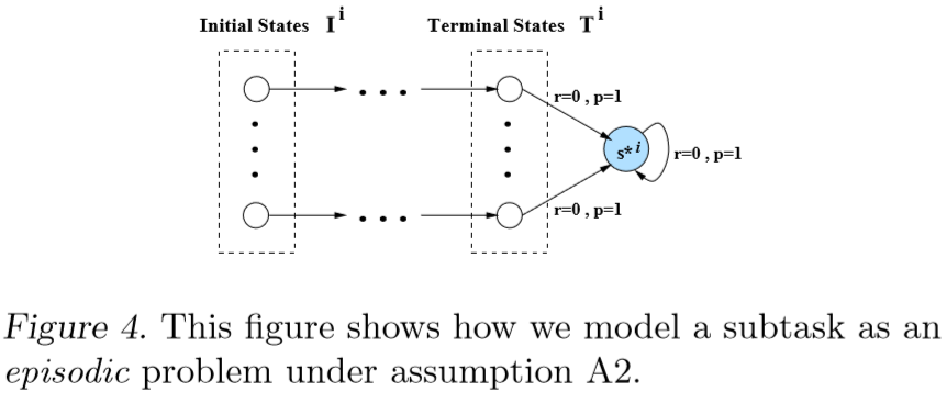
Assumption 2

Subtask Termination

There exists a state s*ⁱ∈ Sⁱsuch that, for every action a ∈ Aⁱ, we have

${\color{Blue} R}^i({\color{Blue} s^*}^i,{\color{Magenta} a})=0$

${\color{Red} P}^i({\color{Blue} s^*}^i \mid {\color{Blue} s^*}^i,{\color{Magenta} a})=1$

and for all stationary polices μⁱ(θⁱ) and all states sⁱ∈ Sⁱ, we have

${\color{Red} P}^i({\color{Blue} s^*}^i, {\color{Blue} N} \mid {\color{Blue} s}, {\color{Red} \mu} ^i ({\color{Red} \theta}^i))>0$

${\color{Blue} N}=\left | {\color{Blue} S}^i \right |$

Under this model, we define a new MDP $M_{\bar{{\color{Red} \pi}}^{\color{Magenta} i}}^{\color{Magenta} i}$ for subtask i transition probabilities:

where

$\bar{\color{Red} {\pi}} ^{\color{Magenta} i}({\color{Blue} s})$ : the probability that subtask i starts at state s.

Let $\mathbb{P}^i_{\bar {\color{Red} \pi}}$ be the set of all transition matrices $P^{\color{Magenta} i}_{\bar{\color{Red} \pi}^{\color{Magenta} i}}(s' \mid s, {\color{red} \mu^i(\theta^i)})$ . We have the following result for subtask i.

Lemma 1

Let assumptions A1 and A2 hold. Then for every $P^i_{\bar {\color{Red} \pi}^i} \in \mathbb{P}^i_{\bar {\color{Red} \pi}}$ , and every state ${\color{Blue} s} \in {\color{Blue} S}^{\color{Magenta} i}$ , we have

$\sum_{n=1}^N P^i_{\bar{\color{Red} \pi}}({\color{Golden} s^*^i}, {\color{Blue} n \mid s}, {\color{Red} \mu}^{\color{Magenta} i}({\color{Red} \theta}^{\color{Magenta} i}))>0$ where

${\color{Blue} N}=\left | {\color{Blue} S}^i \right |$

Lemma 1 is equivalent to assume that the MDP $M_{\bar{{\color{Red} \pi}}^{\color{Magenta} i}}^{\color{Magenta} i}$ is recurrent, i.e., the underlying Markov chain for every policy μⁱ(θⁱ) in this MDP has a single recurrent class and the state s*ⁱis recurrent state.

Performance Measure Definition

Paper defines weighted reward-to-go ${\color{Blue} \chi} ^{\color{Magenta} i}({\color{Red} \theta}^{\color{Magenta} i})$ , the performance measure of subtask i formulated by parameterized policy μⁱ(θⁱ).

Assumption A2 holds

${\color{Blue} \chi}^i(\theta^i)=\sum_{s \in S^i} \bar {\color{Red} \pi}^i(s){\color{Blue} J}^i(s,{\color{Red} \theta}^i)$

where ${\color{Blue} J}^{\color{Magenta} i}({\color{Blue} s},{\color{Red} \theta}^{\color{Magenta} i})$ is reward-to-go of state s.

${\color{Blue} J}{\color{Magenta} ^i}({\color{Blue} s},{\color{Red} \theta}^{\color{Magenta} i})=E_{\theta{\color{Magenta} ^i}}\left [ \ \sum_{k=0}^{T-1} {\color{Blue} R}{\color{Magenta} ^i}({\color{Blue} s}_k,{\color{Red} \theta}{\color{Magenta} ^i}) \mid s_0={\color{Blue} s} \ \right ]$

$J{\color{Magenta} ^i}(s, \theta^{\color{Magenta} i})=E_{\theta{\color{Magenta} ^i}}\left [ \ \sum_{{\color{Red} k}=0}^{T-1} R{\color{Magenta} ^i}( s_{\color{Red} k}, \theta{\color{Magenta} ^i}) \mid s_0= s \ \right ]$

where $T$ is the first future time that state s*ⁱ is visited.

$T=min\left \{ {\color{Red} k} >0 \mid s_{\color{Red} k}={\color{Golden} s^*^i} \right \}$

Optimizing the Weighted Reward-to-Go

Proposition 1

If assumptions A1 and A2 hold

${\color{Golden} \bigtriangledown} {\color{Blue} \chi} ^i({\color{Red} \theta}^i)=E_{\bar \pi^i}\left [T \right ]\sum_{s \in S^i} \sum_{a \in A^i} {\color{Red} \pi}_{\bar \pi^i}^i(s,{\color{Red} \theta}^i) \bigtriangledown {\color{Red} \mu}^i(s,a,\theta^i){\color{Blue} Q}^i(s,a,{\color{Red} \theta}^i)$

Cycle between consecutive visits to recurrent state s*ⁱ = renewal cycle

${\color{Golden} \bigtriangledown} {\color{Blue} \chi}^{\color{Magenta} i}( {\color{Red} \theta} ^{\color{Magenta} i})$ can be estimated over a renewal cycle as

$F_m^i(\theta^i)=\sum_{n=t_m}^{t_{m+1}-1} {\color{Blue} \tilde{Q}}^i(s_n,a_n,\theta^i)\frac{\bigtriangledown \mu^i(s_n,a_n,\theta^i)}{\mu^i(s_n,a_n,\theta^i)}$ (P1)

$\tilde{{\color{Blue} Q}}^i(s_n,a_n,{\color{Red} \theta}^i)=\sum_{k=n}^{{\color{Red} t_{m+1}}-1}{\color{Blue} R}^i(s_n,a_n)$

where t_m is the time of the mth visit at the recurrent state s*ⁱ .

From P1, the paper obtains the following procedure to update the parameter vector along the approximate gradient direction at every time step.

$\begin{align*} {\color{Magenta} z^i}_{k+1}&=\left\{\begin{matrix} 0 & s_k=s^*^i\\ z_k^i+\psi^i(s_k,a_k,\theta_k^i) & otherwise \end{matrix}\right.\\ {\color{Red} \theta^i}_{k+1}&=\theta^i_k+{\color{Golden} \alpha}_k^i{\color{Blue} R}^i(s_k,a_k){\color{Magenta} z^i}_{k+1} \end{align*}$ (P2)

P2 provides an unbiased estimate of ${\color{Golden} \bigtriangledown} {\color{Blue} \chi}^{\color{Magenta} i}( {\color{Red} \theta} ^{\color{Magenta} i})$ . For systems involving a large state space, the interval between visits to state s*ⁱ can be large. As a consequence, the estimate of ${\color{Golden} \bigtriangledown} {\color{Blue} \chi}^{\color{Magenta} i}( {\color{Red} \theta} ^{\color{Magenta} i})$ might have a large variance.

${\color{Golden} \alpha}$ : step size parameter and satisfies the following assumptions.

Assumption 4

${\color{Golden} \alpha}_k$ ‘s are deterministic, nonnegative and satisfy

$\sum_{k=1}^{\infty} {\color{Golden} \alpha}_k =\infty \ and\ \sum_{k=1}^{\infty} {\color{Golden} \alpha}_k^2 < \infty$

Assumption 5

${\color{Golden} \alpha}_k$ ‘s are non-increasing and there exists a positive integer p and a positive scalar A such that

$\sum_{k={\color{Magenta} n}}^{{\color{Magenta} n}+{\color{Red} t}}({\color{Golden} \alpha}_{\color{Magenta} n}-{\color{Golden} \alpha}_k)\leq {\color{DarkGreen} A} {\color{Red} t}^{\color{Blue} p}{\color{Golden} \alpha}_{\color{Magenta} n}^2$

for all positive integers n and t.

The paper has the following convergence result for the iterative procedure in P2 to update the parameters.

Proposition 2

Let assumption A1, A2, A4 and A5 hold, and let $\left ( {\color{Red} \theta}^i_k \right )$ be the sequence of parameter vectors generated by P2. Then, ${\color{Blue} \chi}^i({\color{Red} \theta}_k^i)$ converges and

$lim_{k \to \infty}{\color{Golden} \bigtriangledown} {\color{Blue} \chi}^i({\color{Red} \theta}^i_k)=0$

with probability 1.

Pei

Email Address:

Blog Stats

State Action/Control

Meta

Hierarchical Policy Gradient Algorithms