Decentralized Stabilization for a Class of Continuous-Time Nonlinear Interconnected Systems Using Online Learning Optimal Control Approach

Neural-network-based Online Learning Optimal Control

Decentralized Control Strategy

Cost functions (critic neural networks) – local optimal controllers
Feedback gains to the optimal control policies – decentralized control strategy

Optimal Control Problem (Stabilization)

Hamilton-Jacobi-Bellman (HJB) Equations

Apply Online Policy Iteration Algorithm (construct and train critic neural networks) to solve HJB Equations.

The decentralized control has been a control of choice for large-scale systems because it is computationally efficient to formulate control law that use only locally available subsystem states or outputs.

Though dynamic programming is a useful technique to solve the optimization and optimal control problems, in may cases, it is computationally difficult to apply it because of the curse of dimensionality.

Considering the effectiveness of ADP and reinforcement learning techniques in solving the nonlinear optimal control problem, the decentralized control approach established is natural and convenient.

Notation

$i=1,2,...,N.$ : ith subsystem.

${\color{Blue} x}_i(t)\in \mathbb{R}^{n_i}$ : state vector of the ith subsystem.

${\color{Blue} x}_1,{\color{Blue} x}_2, ...,{\color{Blue} x}_N$ : local states.

${\color{Red} \bar u}_i({\color{Blue} x}_i(t)) \in \mathbb{R}^{m_i}$ : control vector of the ith subsystem.

${\color{Red} \bar u}_1({\color{Blue} x}_1) , {\color{Red} \bar u}_2({\color{Blue} x}_2) , ..., {\color{Red} \bar u}_N({\color{Blue} x}_N)$ : local controls.

${\color{Red} u}_i({\color{Blue} x}_i), i=1,2,...,N$ : control policies.

${\color{Golden} f}_i({\color{Blue} x}_i)$ : nonlinear internal dynamics.

${\color{Magenta} g}_i({\color{Blue} x}_i)$ : input gain matrix.

${\color{Magenta} g}_i(x_i){\color{Magenta} \bar Z}_i(x)$ : interconnected term. Z_i(x)‘s x has no i .

${\color{Golden} R}_i \in \mathbb{R}^{m_i \times m_i}, i=1,2,...,N.$ : symmetric positive definite matrices.

$\rho$ : nonnegative constants.

${\color{Orange} h}_{ij}(x_j)$ : positive semidefinite function.

$Q_i(x_i), i=1,2,...,N.$ : positive definite functions satisfying ${\color{Orange} h}_i(x_i) \leq Q_i(x_i), i=1,2,...,N.$

${\color{Red} \mu}_i({\color{Blue} x}_i)$ : control policy.

$\Omega _i$ : ${\color{Golden} f}_i+{\color{Magenta} g}_i {\color{Red} u}_i$ is Lipshcitz continuous on a set $\Omega _i$ in $\mathbb{R} ^{n_i}$ containing the origin, and the subsystem is controllable in the sense that there exists a continuous control policy on $\Omega _i$ that asymptotically stabilizes the subsystem.

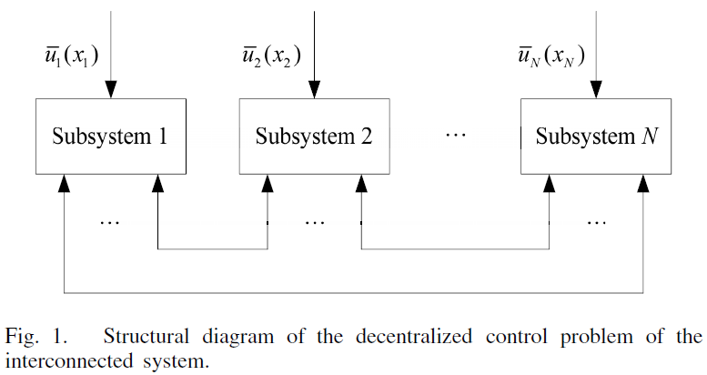
Decentralized Control Problem of the Large-Scale System

Paper studies a class of continuous-time nonlinear large-scale systems: composed of N interconnected subsystems described by

$\begin{align*} \dot{{\color{Blue} x}}_i(t)&={\color{Golden} f}_i \left ( {\color{Blue} x}_i(t) \right ) + {\color{Magenta} g}_i\left ( {\color{Blue} x}_i(t) \right ) \left ( {\color{Red} \bar u}_i ({\color{Blue} x}_i(t)) + {\color{Magenta} \bar Z}_i ({\color{Blue} x}(t))\right )\\ i &=1,2,...,N \end{align*}$ (1)

${\color{Blue} x}_i(0)={\color{Blue} x}_{i0}$ : initial state of the ith subsystem,

Assumption 1: When ${\color{Blue} x}_i=0$ , ith subsystem is equilibrium.

Assumption 2: ${\color{Golden} f}_i({\color{Blue} x}_i)$ and ${\color{Magenta} g}_i({\color{Blue} x}_i)$ are differentiable in arguments with ${\color{Golden} f}_i({\color{Blue} 0})=0$ .

Assumption 3: When ${\color{Blue} x}_i=0$ , the feedback control vector ${\color{Red} \bar u}_i ({\color{Blue} x}_i) =0$ .

${\color{Magenta} Z}_i(x)={\color{Golden} R}_i^{1/2} {\color{Magenta} \bar Z}_i(x)$

where

${\color{Golden} R}_i \in \mathbb{R}^{m_i \times m_i}, i=1,2,...,N.$ : symmetric positive definite matrices.

${\color{Magenta} Z}_i(x) \in \mathbb{R} ^{m_i},i=1,2,...,N.$

are bounded as follows:

$\begin{align*} \left \| {\color{Magenta} Z}_i(x) \right \| &\leq \sum_{j=1}^N \rho _{ij} {\color{Orange} h}_{ij}(x_j), \\ i&=1,2,...,N. \end{align*}$ (2)

Define

$h_{\color{DarkGreen} i}(x_i)=max\left \{ h_{{\color{Red} 1}{\color{DarkGreen} i}}(x_i) , h_{{\color{Red} 2}{\color{DarkGreen} i}}(x_i),...,h_{{\color{Red} N}{\color{DarkGreen} i}}(x_i)\right \}$

then (2) can be formulated as

$\begin{align*} \left \| Z_i(x) \right \| &\leq \sum_{j=1}^N {\color{Blue} \lambda_{ij}}{\color{Orange} h_j(x_j)},\ i=1,2,...,N.\\ \indent where\\ \indent {\color{Blue} \lambda_{ij}} &\geq \frac{\rho_{ij}h_{ij}(x_j)}{{\color{Orange} h_j(x_j)}} \end{align*}$

C1 – Optimal Control of Isolated Subsystems (Framework of HJB Equations)

C2 – Decentralized Control Strategy

Consider the N isolated subsystems corresponding to (1)

$\begin{align*} \dot{{\color{Blue} x}}_i(t)&={\color{Golden} f}_i \left ( {\color{Blue} x}_i(t) \right ) + {\color{Magenta} g}_i\left ( {\color{Blue} x}_i(t) \right ) \left ( {\color{Red} u}_i ({\color{Blue} x}_i(t)) \right )\\ i &=1,2,...,N \end{align*}$ (4)

Find the control policies ${\color{Red} u}_i({\color{Blue} x}_i), i=1,2,...,N$ which minimize the local cost functions

$\begin{align*} {\color{Blue} J}_i({\color{Blue} x}_{i0})&=\int_{0}^{\infty} \left \{ {\color{DarkGreen} Q}_i^2({\color{Blue} x}_i(\tau ))+{\color{Red} u}_i^T({\color{Blue} x}_i(\tau)){\color{Golden} R}_i {\color{Red} u}_i({\color{Blue} x}_i(\tau)) \right \}d\tau \\ i&=1,2,...,N \end{align*}$ (5)

( How to get the equation 5 ? Should Q = Q and R = P, (Q and P ∈ Lyapunov Equation) ? )

to deal with the infinite horizon optimal control problem.

where

$Q_i(x_i), i=1,2,...,N.$ : positive definite functions satisfying

${\color{Orange} h}_i(x_i) \leq Q_i(x_i), i=1,2,...,N.$ (6)

Based on optimal control theory, feedback controls (control policies) must be admissible , i.e., stabilize the subsystmes on $\Omega _i$ , guarantee cost function (5) are finite.

Admissible Control

Definition 1

Consider the isolated subsystem i,

$\begin{align*} {\color{Red} \mu}_i &\in \Psi_i( \Omega_i)\\ {\color{Red} \mu}_i(0) &=0 \\ {\color{Red} u}_i(x_i)&={\color{Red} \mu}_i(x_i)\\ \end{align*}$

For any set of admissible control policies ${\color{Red} \mu}_i \in \Psi_i(\Omega_i), i=1,2,...,N$ , if the associated cost functions

$\begin{align*} {\color{Blue} V}_i(x_{i0})&=\int_{0}^{\infty} \left \{ Q_i^2(x_i(\tau)) + {\color{Red} \mu}_i^T (x_i(\tau)) R_i {\color{Red} \mu}_i(x_i(\tau))\right \}d\tau \\ i&=1,2,...,N. \end{align*}$

(7)

are continuously differentiable, then the infinitesimal versions of (7) are the so-called nonlinear Lyapunov equations

$0=Q^2_i(x_i)+{\color{Golden} \mu_i^T(x_i)R_i\mu_i(x_i)}+ ( \bigtriangledown {\color{Blue} V}_i(x_i))^T \left({\color{Golden} f}_i(x_i))+{\color{Magenta} g}_i(x_i){\color{Red} \mu}_i(x_i) \right )$ (8)

( How to get the equation 8 ? Should Q = Q and R = P, (Q and P ∈ Lyapunov Equation) ? )

where

$\begin{align*} {\color{Blue} V}_i(0) &=0 \\ \bigtriangledown {\color{Blue} V}_i(x_i)&=\frac{\partial {\color{Blue} V}_i(x_i)}{\partial x_i}\\ i&=1,2,...,N. \end{align*}$

———————————-

Lyapunov Equation

Linear Quadratic Lyapunov Theory

Linear Quadratic Lyapunov Theory Notes

Lyapunov Equation

We assume  It follows that .
Continuous-time linear systems: where P, Q satisfy (continuous-time) Lyapunov Equation: 
If P>0, Q>0, then system is (globally asymptotically) stable.
If P>0, Q≥0, and (Q,A) observable, then system is (globally asymptotically) stable.

${\color{Blue} A}^T{\color{Golden} P}+{\color{Golden} P}{\color{Blue} A}+{\color{Magenta} Q}=0$

where A, P, Q ∈ R^{n x n}, and P, Q are symmetric

interpretation: for linear system

$\dot{x}={\color{Blue} A}x$

$V(z)=z^T {\color{Golden} P}z$

$V(z)={\color{Golden}z^T Pz}$

then

$\dot{V}(z)=({\color{Blue} A}z)^T{\color{Golden} P}z+z^T{\color{Golden} P}({\color{Blue} A}z)=-z^T{\color{Magenta} Q}z$

$\dot{V}(z)=({\color{Blue} A}z)^T{\color{Golden} P}z+z^T{\color{Golden} P}({\color{Blue} A}z)={\color{Magenta}-z^T Qz}$

i.e., if ${\color{Golden} z^TPz}$ is the (generalized) energy, then ${\color{Magenta} z^TQz}$ is the associated (generalized) dissipation

Lyapunov Integral

If A is stable there is an explicit formula for solution of Lyapunov equation:

${\color{Golden} P}=\int_{0}^{\infty} e ^{t{\color{Blue} A}^T}{\color{Magenta} Q}e^{t{\color{Blue} A}}dt$

to see this, we note that

$\begin{align*} {\color{Blue} A}^T{\color{Golden} P}+{\color{Golden} P}{\color{Blue} A} &=\int_{0}^{\infty}\left ( {\color{Blue} {\color{Blue} A}}^Te^{t{\color{Blue} A}^T}{\color{Magenta} Q}e^{t{\color{Blue} A}} +e^{t{\color{Blue} A}^T}{\color{Magenta} Q}e^{t{\color{Blue} A}} {\color{Blue} A} \right ) \\ &=\int_{0}^{\infty} \left ( \frac{\mathrm{d} }{\mathrm{d} t}e^{t{\color{Blue} A}^T}{\color{Magenta} Q}e^{t{\color{Blue} A}}\right )dt \\ &=e^{t{\color{Blue} A}^T}{\color{Magenta} Q}e^{t{\color{Blue} A}}\mid_{0}^{\infty} \\ &=-{\color{Magenta} Q} \end{align*}$

Interpretation as cost-to-go

If A is stable, and P is (unique) solution of

${\color{Blue} A}^T{\color{Golden} P}+{\color{Golden} P}{\color{Blue} A}+{\color{Magenta} Q}=0$

, then

$\begin{align*} V(z) &=z^T {\color{Golden} P}z \\ &=z^T \left ( \int_{0}^{\infty} e^{t{\color{Blue} A}^T}{\color{Magenta} Q}e^{t{\color{Blue} A}} dt \right )z \\ &=\int_{0}^{\infty} x(t)^T{\color{Magenta} Q}x(t)dt\\ \end{align*}\\ where \ \dot{x}={\color{Blue} A}x,{\color{Red} x(0)=z}$

thus V(z) is cost-to-go from point z (with no input) and integral quadratic cost function with matrix Q

If A is stable and Q>0, then for each t, $e^{t{\color{Blue} A}^T}{\color{Magenta} Q}e^{t{\color{Blue} A}}>0$ , so

${\color{Golden} P}=\int_{0}^{\infty} e ^{t{\color{Blue} A}^T}{\color{Magenta} Q}e^{t{\color{Blue} A}}dt>0$

meaning: if A is stable,

we can choose any positive definite quadratic form $z^T{\color{Magenta} Q}z$ as the dissipation, i.e., $-\dot V=z^T{\color{Magenta} Q}z$
then solve a set of linear equations to find the (unique) quadratic form $\dot V=z^T{\color{Magenta} Q}z$
V will be positive definite, so it is a Lyapunov function that proves A is stable.

In particular: a linear system is stable if an only if there is a quadratic Layapunov function that proves it.

Evaluating Quadratic Integrals

Suppose $\dot x ={\color{Blue} A}x$ is stable, and define

$J=\int_{0}^{\infty}x(t)^T{\color{Magenta} Q}x(t)dt$

to find J, we solve Lyapunov equation

${\color{Blue} A}^T{\color{Golden} P}+{\color{Golden} P}{\color{Blue} A}+{\color{Magenta} Q}=0$

for P then,

$J=x(0)^T{\color{Golden} P}x(0)$

In other words: we can evaluate quadratic integral exactly, by solving a set of linear equations, without even computing a matrix exponential.

———————————-

Pei

Email Address:

Blog Stats

State Action/Control

Meta

Decentralized Stabilization for a Class of Continuous-Time Nonlinear Interconnected Systems Using Online Learning Optimal Control Approach