Policy Gradient Methods

In summary, I guess because 
1. policy (probability of action) has the style: , 
2. obtain (or let's say 'math trick')  in the objective function (  i.e., value function  )'s gradient equation to 
get an 'Expectation' form for : , 
assign 'ln' to policy before gradient for analysis convenience.

Notation

J(θ): any policy objective function of θ (vector).

$\alpha$ : step-size parameter.

$\triangledown_{\theta}J(\theta)=\begin{pmatrix} \frac{\partial J(\theta)}{\partial \theta_1}\\ .\\ .\\ .\\ \frac{\partial J(\theta)}{\partial \theta_n} \\ \end{pmatrix}$

: policy gradient.

$\triangle \theta = \alpha \triangledown_{\theta}J(\theta)$ : ascending the gradient of the policy.

$\pi_{\theta}(s,a)$ : action policy.

Usually, probability of action looks like:

$\pi_{\theta}(a\mid s, \theta)\doteq \frac{e^{h(s,a,\theta)}}{\sum_b e^{h(s,b,\theta)}}=\frac{e^{\theta^Tx(s,a)}}{\sum_b e^{h(s,b,\theta)}}$ (a)

Soft-max policy, weight actions use linear combination of features x

$\pi_{\theta}(a\mid s, \theta)\doteq \frac{1}{\sigma (s,\theta)\sqrt{2\pi}}e^{-\frac{[a-\mu(s,\theta)]^2}{2\sigma(s,\theta)^2}}$

$\begin{align*} \mu(s,\theta) &\doteq \theta_{\mu}^T x_{\mu}(s)\\ \sigma(s,\theta) &\doteq e^{\theta_{\sigma}^Tx_{\sigma}(s)} \end{align*}$

(b)

continuous action, Gaussian distribution policy

$\begin{align*} \triangledown _{\theta} \left [ \pi_{\theta}(a \mid s,\theta) \right ] &= \pi_{\theta}(a \mid s, \theta)\frac{\triangledown_\theta [ \pi_\theta (a\mid s,\theta) ] }{\pi_\theta(a \mid s, \theta)}\\ &=\pi_\theta(a \mid s, \theta) \triangledown_\theta \left \{ \textup{ln} \left [ \pi_\theta(a \mid s, \theta)\right ] \right \} \end{align*}$

We get score function $\triangledown_\theta \{ \textup{ln} \left [ \pi_\theta(a \mid s, \theta)\right ] \}$ .

For (a)

$\triangledown_\theta\textup{ln} \left [ \pi_\theta(a \mid s, \theta)\right ]=x(s,a)-\texttt{E}_{\pi_{\theta}}[x(s, \cdot )]$

For (b) $\begin{align*} \triangledown_{\theta_{\mu}}\textup{ln} \left [ \pi_\theta(a \mid s, \theta_{\mu})\right ] &=\triangledown_{\theta_{\mu}} \textup{ln} \left [ \frac{1}{\sigma (s,\theta)\sqrt{2\pi}}e^{-\frac{[a-\mu(s,\theta)]^2}{2\sigma(s,\theta)^2}} \right ] \\ &=\triangledown_{\theta_{\mu}} \left [ \textup{ln}1 -\textup{ln} \left [ \sigma(s,\theta)\sqrt{2\pi}\right ] - \frac{[a-\mu(s,\theta)]^2}{2\sigma(s,\theta)^2}\right ]\\ &=0-0-\triangledown_{\theta_{\mu}}\frac{[a-\mu(s,\theta)]^2}{2\sigma(s,\theta)^2}\\ &=-\frac{2[a-\mu(s,\theta)]}{2\sigma(s,\theta)^2}\left [ -\frac{\partial \mu(s,a)}{\partial \theta_{\mu}} \right ] \\ &=-\frac{[a-\mu(s,\theta)]}{\sigma(s,\theta)^2}\left [ -\frac{\partial \theta_\mu^T x_\mu(s)}{\partial \theta_{\mu}} \right ]\\ &=\frac{[a-\mu(s,\theta)]}{\sigma(s,\theta)^2}\left [ x_\mu(s) \right ] \end{align*}$

$\begin{align*} \triangledown_{\theta_{\sigma}}\textup{ln} \left [ \pi_\theta(a \mid s, \theta_{\sigma})\right ] &= \triangledown_{\theta_{\sigma}} \textup{ln} \left [ \frac{1}{\sigma (s,\theta)\sqrt{2\pi}}e^{-\frac{[a-\mu(s,\theta)]^2}{2\sigma(s,\theta)^2}} \right ] \\ &=\triangledown_{\theta_{\sigma}} \left [ \textup{ln}1- \textup{ln} \left [ \sigma(s,\theta)\sqrt{2\pi} \right ] - \frac{[a-\mu(s,\theta)]^2}{2\sigma(s,\theta)^2}\right ] \\ &=0- \frac{1}{\sigma(s,\theta)\sqrt{2\pi}}\sqrt{2\pi}\frac{\partial \sigma(s,\theta)}{\partial \theta_\sigma}+\frac{[a-\mu(s,\theta)]^2}{\sigma(s,\theta)^3} \frac{\partial \sigma(s,\theta)}{\partial \theta_\sigma} \\ &=- \frac{1}{\sigma(s,\theta)}\frac{\partial e^{\theta_\sigma^T x_\sigma(s)}}{\partial \theta_\sigma}+\frac{[a-\mu(s,\theta)]^2}{\sigma(s,\theta)^3} \frac{\partial e^{\theta_\sigma^T x_\sigma(s)}}{\partial \theta_\sigma} \\ \end{align*}$

$\begin{align*} \triangledown_{\theta_{\sigma}}\textup{ln} \left [ \pi_\theta(a \mid s, \theta_{\sigma})\right ] &=-\frac{1}{\sigma(s,\theta)}\sigma(s,\theta)x_{\sigma}(s)+\frac{[a-\mu(s,\theta)]^2}{\sigma(s,\theta)^3}\sigma(s,\theta)x_\sigma(s)\\ &=\left [ \frac{ [a-\mu(s,\theta)]^2}{\sigma(s,\theta)^2} - 1 \right ] x_\sigma(s) \\ \end{align*}$

The results are the same as the equations at the page 336 from Chapter 13. Policy Gradient Methods. Reinforcement Learning: an introduction, 2nd, Richard S. Sutton and Andrew G. Barto.

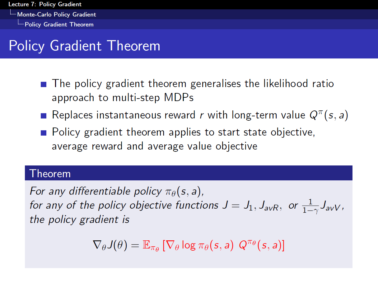
For one-step MDPs:

$J(\theta)=\texttt{E}[r]=\sum_{s\in \texttt{S}}d(s)\sum_{a\in \texttt{A}}\pi_{\theta}(a \mid s)\texttt{R}_{(s,a)}$

$\begin{align*} \triangledown_{\theta}J(\theta) &=\sum_{s\in \texttt{S}}d(s)\sum_{a\in \texttt{A}}\pi_{\theta}(a \mid s)\triangledown_{\theta}\left [ \texttt{ln}\pi_{\theta}(a \mid s) \right ] \texttt{R}_{(s,a)} \\ &=\texttt{E}_{\pi_\theta}\left [\triangledown_{\theta} \texttt{ln}\pi_{\theta}(a\mid s)r \right ] \end{align*}$

$r=\texttt{R}_{(s,a)}$

$\texttt{r:instantaneous reward.}$

For any of the policy objective functions:

$\triangledown_{\theta}J(\theta)=\texttt{E}_{\pi_\theta}\{ \triangledown_\theta \left [\texttt{ln} \pi_\theta (a \mid s)\right ] q_\pi(s,a)\right ] \}$

$q_\pi(s,a)\texttt{:long term value.}$

$\triangle \theta_t=\alpha \triangledown J(\theta)=\alpha \triangledown \left [ \texttt{ln}\pi_\theta(a\mid s,\theta_t) \right ] \texttt{v}_t$

$\texttt{v}_t \texttt{:return, it is an unbiased sample of } q_\pi(s_t,a_t).$

so, we get algorithm for updating θ:

$\theta \leftarrow \theta + \alpha \triangledown_\theta \left [ \texttt{ln} \pi_\theta (a_t \mid s_t) \right ]\texttt{v}_t$

In summary, I guess because 
1. policy (probability of action) has the style: , 
2. obtain (or let's say 'math trick')  in the objective function (  i.e., value function  )'s gradient equation to 
get an 'Expectation' form for : , 
assign 'ln' to policy before gradient for analysis convenience.

Pei

Email Address:

Blog Stats

State Action/Control

Meta

Policy Gradient Methods

Policy Gradient Methods

Last posts