Fourier Transform and Matrix-vector Multiplication

Fourier Transform Math Background and Dot-product Engine Matrix-vector Multiplication Analysis About Software Flow Based On MATLAB

Code is not available online because of Copyright and Academic Secret.

Fourier Transform

${\color{Red} x(t)} {\color{Magenta} \Leftrightarrow } {\color{Blue} X(\omega )}$

K. R. Rao and P. Yip, Discrete cosine transform: algorithms, advantages, applications.

We will start by recalling the definition of the Fourier transform. Given a function x(t) for $-\infty < t< \infty$ , its Fourier transform is given by

${\color{Magenta} X\left ( \omega \right )\equiv F\left [ x\left ( t \right ) \right ]=\left ( \frac{1}{2\pi } \right )^{\frac{1}{2}}\int_{-\infty }^{\infty }x\left ( t \right )e^{-j\omega t}dt}$ ,

subject to the usual existence conditions for the integral. Here, $j=\sqrt{-1}$ , $\omega =2\pi f$ is the radian frequency and $f$ is the frequency in Hertz. The function x(t) can be recovered by the inverse Fourier transform, i.e.,

$x(t)\equiv F^{-1}\left [ X\left ( \omega \right ) \right ]=\left ( \frac{1}{2\pi } \right )^{\frac{1}{2}}\int_{-\infty }^{\infty }X(\omega )e^{j\omega t}d\omega$

If x(t) is defined only for ${\color{Blue} t\geqslant 0}$ , we can construct a function y(t) given by:

${\color{Blue} y(t)= \left\{\begin{matrix} x(t) & t\geqslant 0\\ x(-t) & t\leqslant 0 \end{matrix}\right.}$

Then

${\color{Blue} \begin{align*} F[y(t)] &=\left ( \frac{1}{2\pi } \right )^{\frac{1}{2}} \left \{ \int_{0}^{\infty } x(t)e^{-j\omega t}dt+\int_{-\infty }^{0}x(-t)e^{-j\omega t}dt\right \}\\ &= \left ( \frac{1}{2\pi } \right )^{\frac{1}{2}} \int_{0}^{\infty }x(t)\left [ e^{-j\omega t}+e^{j\omega t} \right ]dt\\ &= \left ( \frac{2}{\pi } \right )^{\frac{1}{2}} \int_{0}^{\infty }x(t)cos(\omega t)dt \end{align*}}$

We can now define this as the Fourier cosine transform (FCT) of x(t) given by

${\color{Purple} X_{c}(\omega )\equiv F_{c}\left [ x(t) \right ]=\left ( \frac{2}{\pi } \right )\int_{0}^{\infty }x(t)cos(\omega t)dt}$

Noting that $X_{c}\left ( \omega \right )$ is an even function of $\omega$ , we can apply the Fourier inversion to ${\color{Blue} F[y(t)]}$ to obtain

$y(t)=x(t)\equiv F_{c}^{-1}\left [ X_{c}\left ( \omega \right ) \right ]=\left ( \frac{2}{\pi } \right )^{\frac{1}{2}}\int_{0}^{\infty }X_{c}\left ( \omega \right )cos(\omega t)d\omega$

$(t\geqslant 0)$

The convolution property: Recall that the convolution of two functions x(t) and y(t) is given by

$x(t)\ast y(t)\equiv \int_{0}^{\infty }x(t-u)y(u)du$

The Fourier cosine transform of x*y is given by

$\begin{align*} F_{c}\left [ x(t) \ast y(t)\right ] &=\left ( \frac{2}{\pi} \right )\int_{0}^{\infty}\int_{0}^{\infty}x(t-u)y(u) du \ cos(\omega t) dt \\&=\left ( \frac{\pi}{2} \right )^{\frac{1}{2}}\left [ X_{c}(\omega ) Y_c(\omega) - X_s(\omega)Y_s(\omega)\right ] \end{align*}$

where $F_{s}$ denotes the Fourier sine transform (FST) given by

$F_{s}[x(t)]\equiv \left ( \frac{2}{\pi} \right )^{\frac{1}{2}}\int_{0}^{\infty}x(t)sin(\omega t)dt$

${\color{Purple} X_{c}(\omega )\equiv F_{c}\left [ x(t) \right ]=\left ( \frac{2}{\pi } \right )\int_{0}^{\infty }x(t)cos(\omega t)dt}$

has a kernel given by

$K_c(\omega,t)=cos(\omega t)$

Let $\omega_m=2\pi m {\color{DarkOrange} \delta f}$ and $t_n=n{\color{DarkOrange} \delta t}$ be the sampled angular frequency and time, where ${\color{DarkOrange} \delta f}$ and ${\color{DarkOrange} \delta t}$ represent the unit sample intervals for frequency and time, respectively; m and n are integers.

$\begin{align*} K_c(\omega_m, t_n)&=K_c(2\pi m {\color{DarkOrange} \delta f}, n {\color{DarkOrange}\delta t}) \\ &=cos(2\pi mn {\color{DarkOrange}\delta f \delta t}) \\ &= K_c(m,n) \end{align*}$

If we further let ${\color{DarkOrange} \delta f \delta t = \frac{1}{2N}}$ where N is an integer, we have

${\color{Orchid} K_c(m,n)=cos\left ( \frac{\pi mn}{N} \right )}$

which represents a discretized Fourier cosine kernel. But, it is far simpler, both mathematically and conceptually, to regard the discrete kernel as elements in an (N + 1) by (N + 1) transform matrix. Let his matrix be denoted by [M]. Then, the mnth element of this matrix is

${\color{Orchid} [M]_{mn}=cos \left ( \frac{\pi m n}{N} \right )}$

${\color{Orchid} m,n=0,1, ..., N.}$

When [M] is applied to a column vector $x=[x(0), x(1), ...,x(N)]^T$ , we obtain the vector

$X=[X(0), X(1),...,X(N)]^T$ such that

$X=[M]x$

where

$X(m)=\sum_{n=0}^{N}{\color{Orchid} cos\left (\frac{\pi mn}{N} \right )}x(n)$

$m=0,1,...,N.$

DCT-II:

$[C_N^{II}]_{mn}=\left ( \frac{2}{N} \right )^\frac{1}{2} \left [k_m cos \left ( \frac{m(n+ \frac{1}{2}) \pi}N \right ) \right ]$

$m,n=0, 1, ..., N-1$

where

$\begin{align*} k_j &=1 \ \ \ if \ j\neq 0 \ or \ N \\ &=\frac{1}{\sqrt{2}} \ \ if \ j=0 \ or \ N \end{align*}$

Fourier cosine transform (FCT) of x(t) given by

${\color{Purple} X_{c}(\omega )\equiv F_{c}\left [ x(t) \right ]=\left ( \frac{2}{\pi } \right )\int_{0}^{\infty }x(t)cos(\omega t)dt}$

DCT-II Forward:

${\color{Orchid} X^{C(2)}(m)=\left ( \frac{2}{N} \right )^\frac{1}{2} k_m \sum_{n=0}^{N-1} x(n)cos \left [ \frac{m(n+ \frac{1}{2}) \pi}N \right ]}$

$m=0, 1, ..., N-1$

where

$\begin{align*} k_j &=1 \ \ \ if \ j\neq 0 \ or \ N \\ &=\frac{1}{\sqrt{2}} \ \ if \ j=0 \ or \ N \end{align*}$

DCT-II Inverse:

$x(n)=\left ( \frac{2}{N}\right )^{\frac{1}{2}} \sum_{m=0}^{N-1} k_m X^{C(2)}(m) cos \left [ \frac {m(n+\frac{1}{2})\pi}{N} \right ]$

$n=0, 1, ..., N-1$

where

$\begin{align*} k_j &=1 \ \ \ if \ j\neq 0 \ or \ N \\ &=\frac{1}{\sqrt{2}} \ \ if \ j=0 \ or \ N \end{align*}$

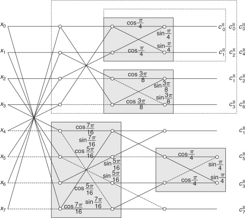
Signal flow graph for DCT-II, N=8.

Discrete Fourier Transform (DFT) converts the sampled signal or function from its original domain (order of time or position) to the frequency domain. It is regarded as the most important discrete transform and used to perform Fourier analysis in many practical applications including mathematics, digital signal processing and image processing.

Discrete cosine transform (DCT) is a Fourier-related transform similar to DFT, but using only real numbers. Comparing to DFT, DCT has two strong advantages: first, it is much easier to compute, second and more important, it has nice energy compaction.

Analysis About Software Flow Based On MATLAB

Accelerating Discrete Fourier Transforms with dot-product engine

Code and test images @github private repository

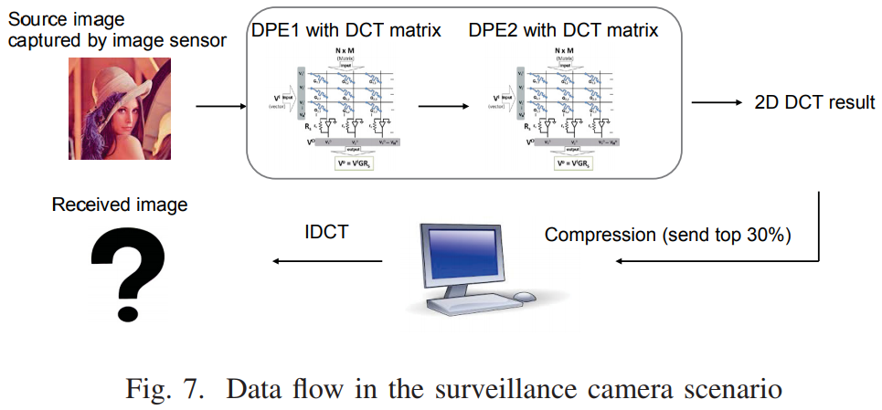
I analyze the software flow without compression from the paper.

————————————————————————————————————-

———————– Analyze DPE based on Discrete Cosine Transform ———————–

MATLAB function dctmtx generates DCT matrix – conductance:

https://www.mathworks.com/help/images/ref/dctmtx.html

MCA DCT matrix for DCT result

D: output of MATLAB function ‘dctmtx’

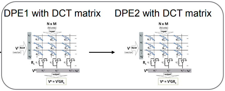
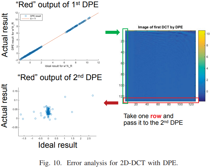
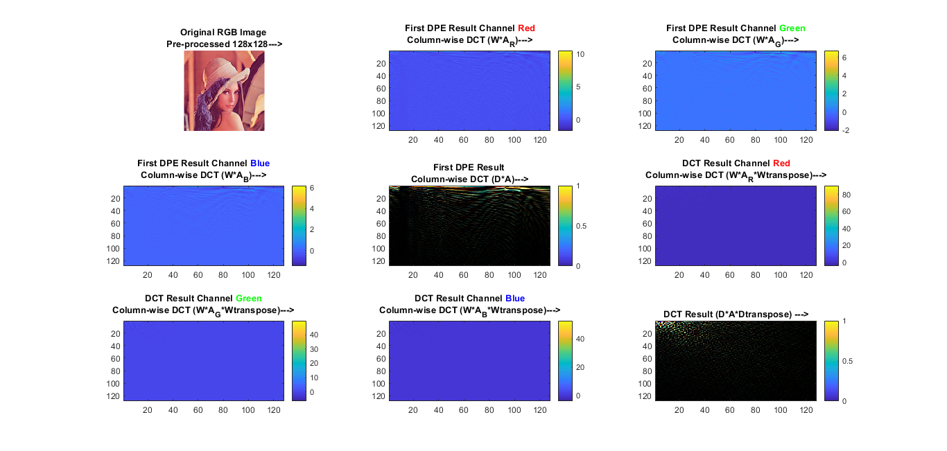
Map D to MCA conductance on the left for the DCT of the columns of Image: D * A (DPE1)

Map D’ to MCA conductance on the right for the DCT of the rows of Image: A * D’ (DPE2)

D = dctmtx(n) returns the n-by-n discrete cosine transform (DCT) matrix, which you can use to perform a 2-D DCT on an image. (dct = D*A *D’)

2D DCT result: dct = D*A * D’

IDCT result: IDCT = D’ * dct * D

If you have an n-by-n image, A, then D*A is the DCT of the columns of A and D'*A is the inverse DCT of the columns of A.
The two-dimensional DCT of A can be computed as D*A *D'. This computation is sometimes faster than using dct2, especially if you are computing a large number of small DCTs, because D needs to be determined only once.For example, in JPEG compression, the DCT of each 8-by-8 block is computed. To perform this computation, use dctmtx to determine D, and then calculate each DCT using D*A *D' (where A is each 8-by-8 block). This is faster than calling dct2 for each individual block.

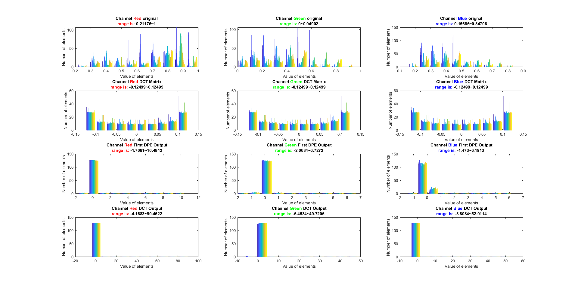
Software Flow Output

Please refer to the results below. Three channels from original RGB image range is [0,1], and IDCT range is [0,1] too, however, DCT matrix has negative or ~90 value.

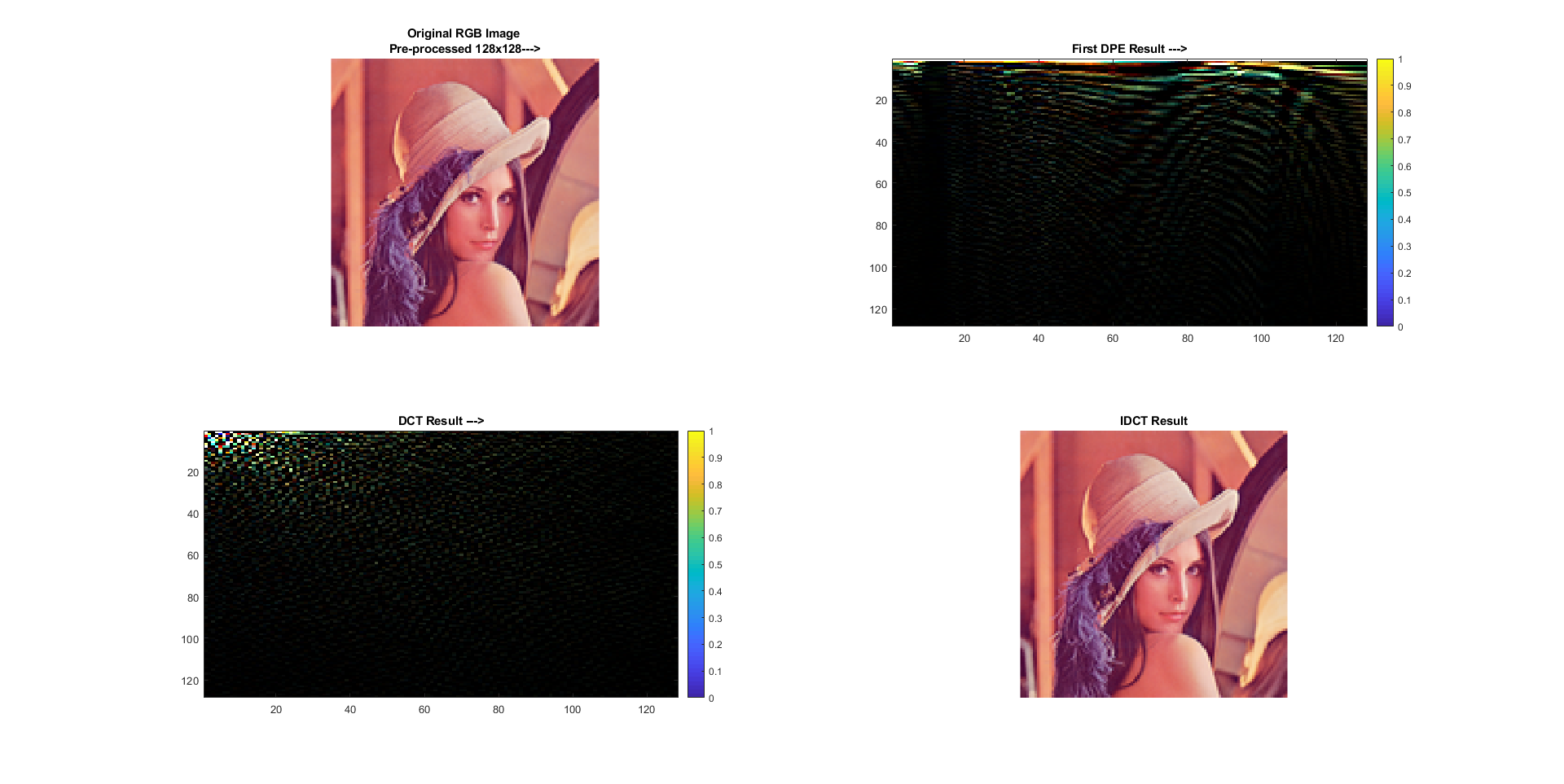
Channel Red Green Blue First DPE and DCT Output without Circuit Simulation

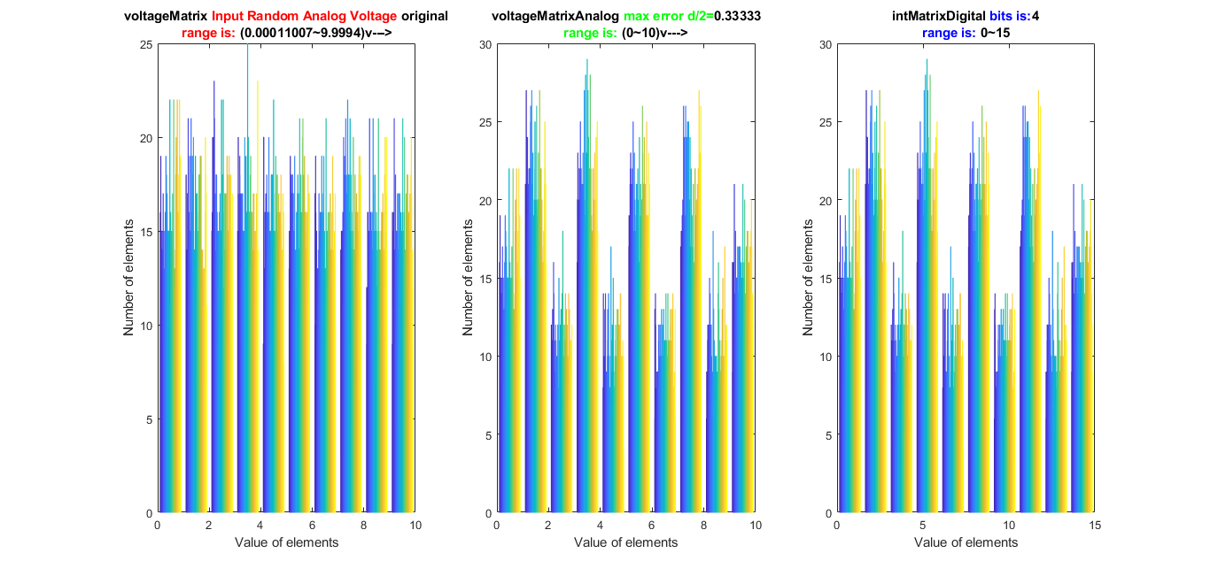
Error Analysis

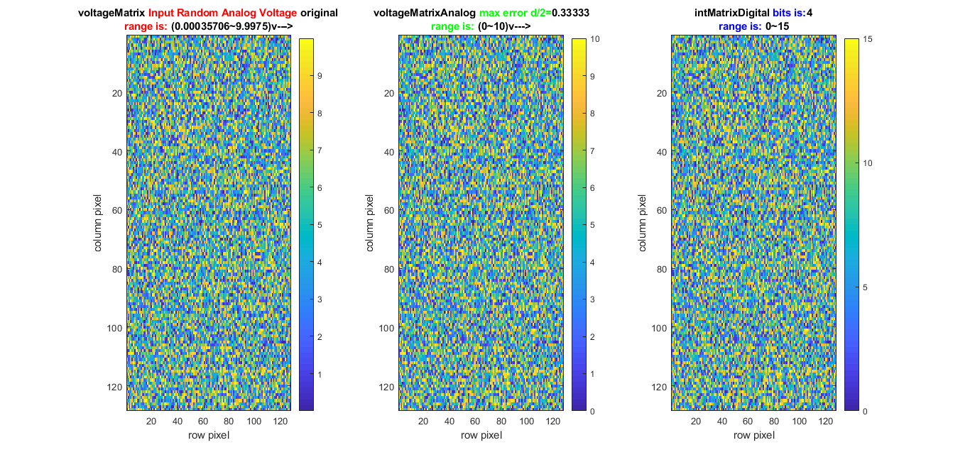
Simulate quantization error from ADC, i.e., the error caused during $x \to x_q$ ,
Then, analyze error of Y in $w \cdot x_q =y$ .
For ADC, voltage criteria discrete delta $d=\frac{V_{max}-V_{min}}{2^{bits}-1}$ , $Error_{max} = \frac{d}{2}$ .

Additional Information Below

Syntax D = dctmtx(n)

Description

D = dctmtx(n) returns the n-by-n discrete cosine transform (DCT) matrix, which you can use to perform a 2-D DCT on an image. (dct = D*A *D’)

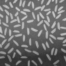
Example: dctmtx

A = im2double(imread(‘rice.png’));

%return 256×256 double

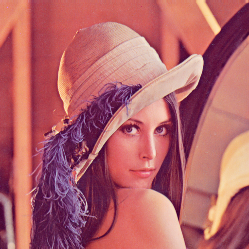
A = im2double(imread(‘lena_std.tif’));

%return 512×512x3 double

but

D = dctmtx(size(A,1));

%return 512×512 no mater original image is gray or color.

Matlab Code (Wrong for RGB Image)

I can’t directly process RGB color image in this way. I need to partition it into three 512×512 matrices, process and recombine.

clear all;

A=im2double(imread(‘lena_std.tif’));
%return 512x512x3 double for color
imshow(A)
sizeA_1=size(A,1)
%return 512.

D = dctmtx(size(A,1));
%Calculate the discrete cosine transform matrix.
%return 512×512 no mater the original image is gray or color.

dct = D.*A.*D’;
%Multiply the input image A by D to get the DCT of the columns of A,
%and by D’ to get the inverse DCT of the columns of A.
%return 512x512x3 double for color.

%If you have an n-by-n image, A, then D*A is the DCT of the columns of A and D’*A is the inverse DCT of the columns of A.

imshow(dct)

Result:

Pei

Email Address:

Blog Stats

State Action/Control

Meta

Fourier Transform and Matrix-vector Multiplication

Fourier Transform Math Background and Dot-product Engine Matrix-vector Multiplication Analysis About Software Flow Based On MATLAB

Fourier Transform

Analysis About Software Flow Based On MATLAB

MATLAB function dctmtx generates DCT matrix – conductance:

Software Flow Output

Channel Red Green Blue First DPE and DCT Output without Circuit Simulation

Error Analysis

Additional Information Below

Syntax D = dctmtx(n)

Matlab Code (Wrong for RGB Image)

I can’t directly process RGB color image in this way. I need to partition it into three 512×512 matrices, process and recombine.

Last posts