Fourier Transform and Matrix-vector Multiplication


K. R. Rao and P. Yip, Discrete cosine transform: algorithms, advantages, applications.


We will start by recalling the definition of the Fourier transform. Given a function x(t) for -\infty < t< \infty, its Fourier transform is given by

{\color{Magenta} X\left ( \omega \right )\equiv F\left [ x\left ( t \right ) \right ]=\left ( \frac{1}{2\pi } \right )^{\frac{1}{2}}\int_{-\infty }^{\infty }x\left ( t \right )e^{-j\omega t}dt},

subject to the usual existence conditions for the integral. Here, j=\sqrt{-1}\omega =2\pi f is the radian frequency and f is the frequency in Hertz. The function x(t) can be recovered by the inverse Fourier transform, i.e.,

x(t)\equiv F^{-1}\left [ X\left ( \omega \right ) \right ]=\left ( \frac{1}{2\pi } \right )^{\frac{1}{2}}\int_{-\infty }^{\infty }X(\omega )e^{j\omega t}d\omega

If x(t) is defined only for {\color{Blue} t\geqslant 0}, we can construct a function y(t) given by:

{\color{Blue} y(t)= \left\{\begin{matrix} x(t) & t\geqslant 0\\ x(-t) & t\leqslant 0 \end{matrix}\right.}

Then

{\color{Blue} \begin{align*} F[y(t)] &=\left ( \frac{1}{2\pi } \right )^{\frac{1}{2}} \left \{ \int_{0}^{\infty } x(t)e^{-j\omega t}dt+\int_{-\infty }^{0}x(-t)e^{-j\omega t}dt\right \}\\ &= \left ( \frac{1}{2\pi } \right )^{\frac{1}{2}} \int_{0}^{\infty }x(t)\left [ e^{-j\omega t}+e^{j\omega t} \right ]dt\\ &= \left ( \frac{2}{\pi } \right )^{\frac{1}{2}} \int_{0}^{\infty }x(t)cos(\omega t)dt \end{align*}}

We can now define this as the Fourier cosine transform (FCT) of x(t) given by

{\color{Purple} X_{c}(\omega )\equiv F_{c}\left [ x(t) \right ]=\left ( \frac{2}{\pi } \right )\int_{0}^{\infty }x(t)cos(\omega t)dt}

Noting that X_{c}\left ( \omega \right ) is an even function of \omega, we can apply the Fourier inversion to {\color{Blue} F[y(t)]} to obtain

y(t)=x(t)\equiv F_{c}^{-1}\left [ X_{c}\left ( \omega \right ) \right ]=\left ( \frac{2}{\pi } \right )^{\frac{1}{2}}\int_{0}^{\infty }X_{c}\left ( \omega \right )cos(\omega t)d\omega

(t\geqslant 0)

The convolution property: Recall that the convolution of two functions x(t) and y(t) is given by

x(t)\ast y(t)\equiv \int_{0}^{\infty }x(t-u)y(u)du

The Fourier cosine transform of x*y is given by

\begin{align*} F_{c}\left [ x(t) \ast y(t)\right ] &=\left ( \frac{2}{\pi} \right )\int_{0}^{\infty}\int_{0}^{\infty}x(t-u)y(u) du \ cos(\omega t) dt \\&=\left ( \frac{\pi}{2} \right )^{\frac{1}{2}}\left [ X_{c}(\omega ) Y_c(\omega) - X_s(\omega)Y_s(\omega)\right ] \end{align*}

where F_{s} denotes the Fourier sine transform (FST) given by

F_{s}[x(t)]\equiv \left ( \frac{2}{\pi} \right )^{\frac{1}{2}}\int_{0}^{\infty}x(t)sin(\omega t)dt


{\color{Purple} X_{c}(\omega )\equiv F_{c}\left [ x(t) \right ]=\left ( \frac{2}{\pi } \right )\int_{0}^{\infty }x(t)cos(\omega t)dt}

has a kernel given by

K_c(\omega,t)=cos(\omega t)

Let \omega_m=2\pi m {\color{DarkOrange} \delta f} and t_n=n{\color{DarkOrange} \delta t} be the sampled angular frequency and time, where {\color{DarkOrange} \delta f} and {\color{DarkOrange} \delta t} represent the unit sample intervals for frequency and time, respectively; m and n are integers.

\begin{align*} K_c(\omega_m, t_n)&=K_c(2\pi m {\color{DarkOrange} \delta f}, n {\color{DarkOrange}\delta t}) \\ &=cos(2\pi mn {\color{DarkOrange}\delta f \delta t}) \\ &= K_c(m,n) \end{align*}

If we further let {\color{DarkOrange} \delta f \delta t = \frac{1}{2N}} where N is an integer, we have

{\color{Orchid} K_c(m,n)=cos\left ( \frac{\pi mn}{N} \right )}

which represents a discretized Fourier cosine kernel. But, it is far simpler, both mathematically and conceptually, to regard the discrete kernel as elements in an (N + 1) by (N + 1) transform matrix. Let his matrix be denoted by [M]. Then, the mnth element of this matrix is

{\color{Orchid} [M]_{mn}=cos \left ( \frac{\pi m n}{N} \right )}

{\color{Orchid} m,n=0,1, ..., N.}

When [M] is applied to a column vector x=[x(0), x(1), ...,x(N)]^T, we obtain the vector

X=[X(0), X(1),...,X(N)]^T such that

X=[M]x

where

X(m)=\sum_{n=0}^{N}{\color{Orchid} cos\left (\frac{\pi mn}{N} \right )}x(n)

m=0,1,...,N.


DCT-II:

[C_N^{II}]_{mn}=\left ( \frac{2}{N} \right )^\frac{1}{2} \left [k_m cos \left ( \frac{m(n+ \frac{1}{2}) \pi}N \right ) \right ]

m,n=0, 1, ..., N-1

where

\begin{align*} k_j &=1 \ \ \ if \ j\neq 0 \ or \ N \\ &=\frac{1}{\sqrt{2}} \ \ if \ j=0 \ or \ N \end{align*}


Fourier cosine transform (FCT) of x(t) given by

{\color{Purple} X_{c}(\omega )\equiv F_{c}\left [ x(t) \right ]=\left ( \frac{2}{\pi } \right )\int_{0}^{\infty }x(t)cos(\omega t)dt}

DCT-II Forward:

{\color{Orchid} X^{C(2)}(m)=\left ( \frac{2}{N} \right )^\frac{1}{2} k_m \sum_{n=0}^{N-1} x(n)cos \left [ \frac{m(n+ \frac{1}{2}) \pi}N \right ]}

m=0, 1, ..., N-1

where

\begin{align*} k_j &=1 \ \ \ if \ j\neq 0 \ or \ N \\ &=\frac{1}{\sqrt{2}} \ \ if \ j=0 \ or \ N \end{align*}

DCT-II Inverse:

x(n)=\left ( \frac{2}{N}\right )^{\frac{1}{2}} \sum_{m=0}^{N-1} k_m X^{C(2)}(m) cos \left [ \frac {m(n+\frac{1}{2})\pi}{N} \right ]

n=0, 1, ..., N-1

where

\begin{align*} k_j &=1 \ \ \ if \ j\neq 0 \ or \ N \\ &=\frac{1}{\sqrt{2}} \ \ if \ j=0 \ or \ N \end{align*}


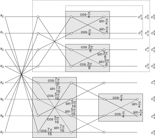
Signal flow graph for DCT-II, N=8.


Discrete Fourier Transform (DFT) converts the sampled signal or function from its original domain (order of time or position) to the frequency domain. It is regarded as the most important discrete transform and used to perform Fourier analysis in many practical applications including mathematics, digital signal processing and image processing.

Discrete cosine transform(DCT) is a Fourier-related transform similar to DFT, but using only real numbers. Comparing to DFT, DCT has two strong advantages: first, it is much easier to compute, second and more important, it has nice energy compaction.


MATLAB function dctmtx generates DCT matrix – conductance:

https://www.mathworks.com/help/images/ref/dctmtx.html


Accelerating Discrete Fourier Transforms with dot-product engine
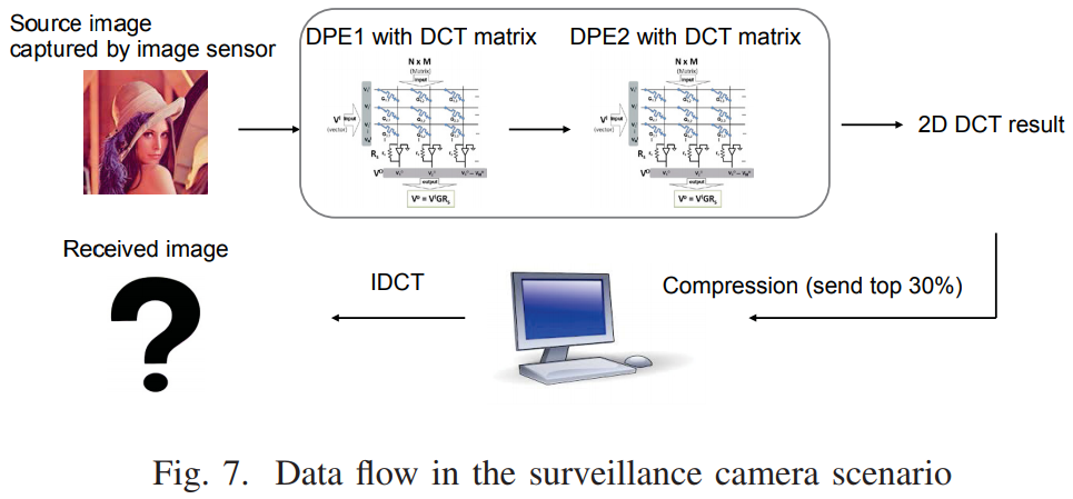
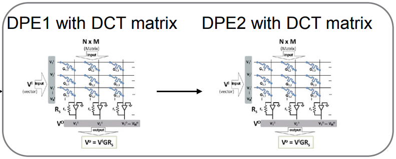
Fig. 1

Fig. 2

MATLAB dctmtx generates the DCT matrix. Map DCT matrix to conductance, i.e., output of MATLAB function ‘dctmtx’ equal/similar to DCT matrix in Fig. 2.

Convolution can be converted to matrix multiplications, for example, DCT.


Sidebar