In empirical sciences, theories can be sorted into three categories with ascending gain of knowledge: empirical, semi-empirical and ab initio. Their difference can best be explained by an example: In astronomy the movement of all planets was known since ancient times. By pure observation astronomers could predict where in the sky a certain planet would be at a given time. They had the knowledge of how they moved but actually no clue why they did so. Their knowledge was purely empirical, meaning purely based on observation. Kepler became the first to develop a model by postulating that the sun is the center of the planetary system and the planet’s movement is controlled by her. Since Kepler could not explain why the planets would be moved by the sun, he had to introduce free parameters which he varied until the prediction of the model matched the observations. This is a so-called semi-empirical model. But it was not until Newton who with his theory of gravity could predict the planets movements without any free parameters or assumptions but purely by an ab initio, latin for “from the beginning”, theory based on fundamental principles of nature, namely gravity. As scientists are quite curious creatures, they always want to know not only how things work but also why they work this way. Therefore, developing ab initio theories is the holy grail in every discipline.
Luckily, in quantum mechanics the process of finding ab initio theories has been strongly formalized. This means that if we want to know the property of a system, for example its velocity, we just have to kindly ask the system for it. This is done by applying a tool, the so-called operator, belonging to the property of interest on the function describing the system’s current state. The result of this operation is the property we are interested in. Think of a pot of water. We want to know its temperature? We use a tool to measure temperature, a thermometer. We want to know its weight? We use the tool to measure its weight, a scale. An operator is a mathematical tool which transforms mathematical functions and provides us with the functions property connected to the operator. Think of the integral sign which is an operator too. The integral is just the operator of the area under a function and the x-axis.
The problem is, how do we know the above mentioned function describing the system’s state? Fortunately, smart people developed a generic way to answer this problem too: We have to solve the so-called Schrödinger equation. Writing down this equation is comparably easy, we just need to know the potentials of all forces acting on the system and we can solve it. Well, if we can solve it. It can be shown that analytical solutions, that means solutions which can be expressed by a closed mathematical expression, only exist for very simple systems, if at all. For everything else numerical approaches have to be applied. While they still converge towards the exact solution, this takes a lot of computational time. The higher the complexity of the system, the more time it takes. So for complex systems even the exact numerical approach quickly becomes impractical to use. One way out of this misery is simplification. With clever assumptions about the system, based on its observation one can drastically reduce the complexity of the calculations. With this approach, we are able to, within reasonable time, find solutions for the problem which are not exact, but exact within a certain error range.
Another way to find a solution for these complex problems is getting help from one of nature’s most powerful and mysterious principles: chance. The problem of the numerical exact solving approach is that it has to walk through an immensely huge multidimensional space, spanned by the combinations of all possible interactions between all involved particles. Think billions of trillions times billions of trillions. By using a technique called Random Walking the time to explore this space can be significantly reduced. Again, let’s take an example: Imagine we want to know how many trees grow in a forest. The exact solution would be dividing the forest into a grid of e.g., 1 square foot, and counting how many trees are in each square. A random walk would start in the forest center. Then we randomly choose a direction and a distance to walk before counting the trees in the resulting square. If we repeat this just long enough we eventually will have visited every square, therefore knowing the exact number, meaning the random walk converges towards the exact result. By having many people starting together and doing individual random walks stopping when their results deviation is below a certain threshold a quite accurate approximation can be obtained in little time.
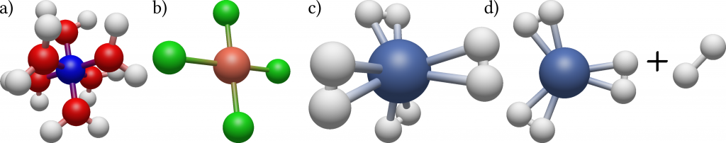
Columbia postdoc Benjamin Rudshteyn and his colleagues developed a very efficient algorithm based on this method specifically tailored for calculating molecules containing transition metals such as copper, niobium or gold. While being ubiquitous in biology and chemistry, and playing a central role in important fields such as the development of new drugs or high-temperature superconductors, these molecules are difficult to treat both experimentally and theoretically due to their complex electronic structures. They tested their method by calculating for a collection of 34 tetrahedral, square planar, and octahedral 3D metal-containing complexes the energy needed to dissociate a part of the molecule from the rest. For this, precise knowledge of the energy states of both the initial molecule and the products is needed. By comparing their results with precise experimental data and results of conventional theoretical methods they could show that their method results in at least two times increased accuracy as well as increased robustness, meaning little variation in the statistical uncertainty between the different complexes.
While still requiring the computational power of modern supercomputers, their findings push the boundaries of the size of transition metal containing molecules for which reliable theoretical data can be produced. These results can then be used as an input to train methods using approximations to further reduce the computational time needed for the calculations.
Dr. Benjamin Rudshteyn is currently a postdoc in the Friesner Group of Theoretical Chemistry, lead by Prof. Dr. Richard A. Friesner, in the Department of Biological Sciences at Columbia University.